| How To Draw Einstein's Face Parametrically |
| Written by Mike James | ||||||||
| Thursday, 19 July 2018 | ||||||||
Page 4 of 4
Convert to rationalsThe next step is to perform the conversion to rationals on A and P. The only real difference is that these are lists rather than scalar values and you can't simply apply the constructor to the list. The solution is to use the map function with a lambda function:
The first instruction applies the constructor to convert the list A into a list of Fraction objects. Next we use the map function to call the limit_denominator method on each of the members of the list. This can't be done directly but its easy to write a lambda function that does the job. At this point we have a set of rational approximations to each term in the form or a list. We can do the same thing to P:
Now we have all of the numeric constants we need all that remains is to build up the terms of the formula as a string. At first however we work with a list of strings and then put the whole lot together with plus signs between. The following is the process broken down into small steps. First we convert the list of adjusted amplitudes into a list of strings:
Next we need to concatenate "*np.sin(" onto the right of each of the strings in s. We can't do this using map because the concatenation operator isn't available as a function. However we can turn it into one and again using a lambda is the easiest way to do this:
You can see that there is a pattern here. If the function accepts a list argument then simply apply it. If it only accepts a scalar then use map to apply it to the list. If it needs some parameters then create a lambda function and apply that using map. All that we need to do now is add the expression that should be inside the brackets sin() :
This looks complicated but it is simply a map using three lists, s, P and a range from 1 to len(P)+1 to supply values for the three parameters a,b and c in the lambda. Now the only thing left is to join all of the terms in the list together with a "+ between each one:
and to remember to put the A0 term into the start of the expression:
This gives us a string that is the formula that we need using t as the variable. Putting this all together as a function:
Of course many of the above statements could be combined to produce a more compact function - but it is better to get something working first. So how do you use this function? In ways that are very similar to the Mathematica code.
The variable xf now contains a string that implements the formula we want:
and getting the formula for y is just as easy:
Now we would like to plot them to see what they look like. The plot range is:
and all we have to do is evaluate xf and yf for each value in ts to create two lists. The easiest way to do this is to use another lambda within a map:
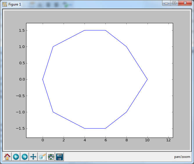
Notice that you don't need to use the parameter t in the lambda function as it is already used within the strings being evaluated. Finally we can plot the result:
If you are using Python 2.7 then you will be disappointed at the result. The reason is that all of the fractions like 356/831 are being evaluated using integer arithmetic. This isn't the case in Python 3 and to update Python 2.7 to this behavior you need to add:
Now it should all work.
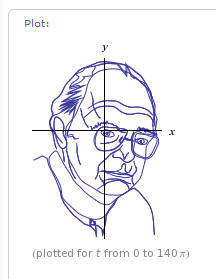
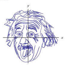
Notice that as the Python plot only draws the points where the series is exact and then joins them with straight lines you don't see the smoothed distortion caused by using the DFT coefficients to interpolate between the points. Where Next?This is almost the complete story but not quite. You now have the tools to create closed parametric curves that match any shape you care to digitize. However the drawings at Wolfram Alpha have many curves not just one. How is this done? The answer is that if you create a curve to work between 0 and 1 and plot it between 0 and 2 you will see two copies of the curve in the same location. The curve is periodic so 0 to 1 or 1 to 2 or 3 to 4 all plot the same curve. So all you have to do is digitize and convert two curves say and plot the first in 0 to 1 and the second in the range 1 to 2 using f1(t)tophat(0,1)+f2(t)tophat(1,2) where tophat(a,b) is a function that is zero except in the range a to b. where it is one. You can see that this results in plotting f1 and then f2. If you look at the Wolfram Alpha examples you will see various theta functions scattered though the plots. These are step functions and two of them together can be used to create a tophat function. What you have to do is digitize each curve that you want for your drawing and then put them all together with the correct tophat functions to create the final result. You could even automate this stage - but I've had enough fun getting this far even though there is more to do. As a final observation, notice that you can also drop terms from the DFT that correspond to high frequencies to make the calculation faster and to smooth the final result. I end with my second favourite parametric portrait:
(See here for a photographic portrait)
If you would like the source code of this project visit the CodeBin. Related Articles:Understanding the Fourier Transform Creating The Python UI With Tkinter Donald Knuth and the Art of Programming
Comments
or email your comment to: comments@i-programmer.info
To be informed about new articles on I Programmer, sign up for our weekly newsletter, subscribe to the RSS feed and follow us on Twitter, Facebook or Linkedin.

|
||||||||
| Last Updated ( Friday, 20 July 2018 ) |