| Multitasking |
| Written by Harry Fairhead | |||
| Friday, 10 June 2022 | |||
Page 1 of 2 We take multitasking for granted now but it was a difficult technology to get right - and still is. We take a look at how it all developed and at the variations on the basic idea.
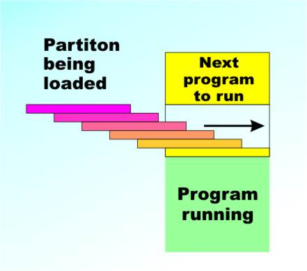
It didn’t take long for the early computer users to realize that the machine had more power than they could actually use. It may have taken hours for one of the early machines to chug its way through a big program, but as soon as it turned its attention to input/output tasks there was lots of time where it just had to sit waiting doing the computer equivalent of contemplating its navel. For example, suppose a computer can obey one million instructions per second – not unreasonable as modern machines reach much higher rates. Now think about an external world operation such as printing a character on paper at say 10 characters per second. The machine cannot start printing the next character until the current one has completed so it generally has to wait 1/10th of a second to execute a single output instruction. In that 1/10th of a second it could have obeyed 100,000 other instructions – a sizeable program. The point is that whenever a computer interacts with the outside world it has to wait and it has time to spare. For the early users computer time was in such short supply that they couldn’t bear to see it go to waste and so multiprocessing was developed. At first this was a fairly primitive mechanism. A typical mainframe machine would be fitted out with more than enough memory to run a typical program – 1MByte say (a lot of memory at the time). Then during the day this 1MByte would be divided up into a number of “partitions”, two small ones, a medium and a large. Programs would then be read into each partition and the processor would run whichever one was ready to go. This was the “batch” processing system that worked so well for so long. Users submitted programs using stacks of punched cards and collected their output, on paper of course, later, often much later typically the next day. The whole point of the batch processing system was to keep the processor well fed with nourishing code and the order in which the programs were run was determined by how best to keep the partitions filled.
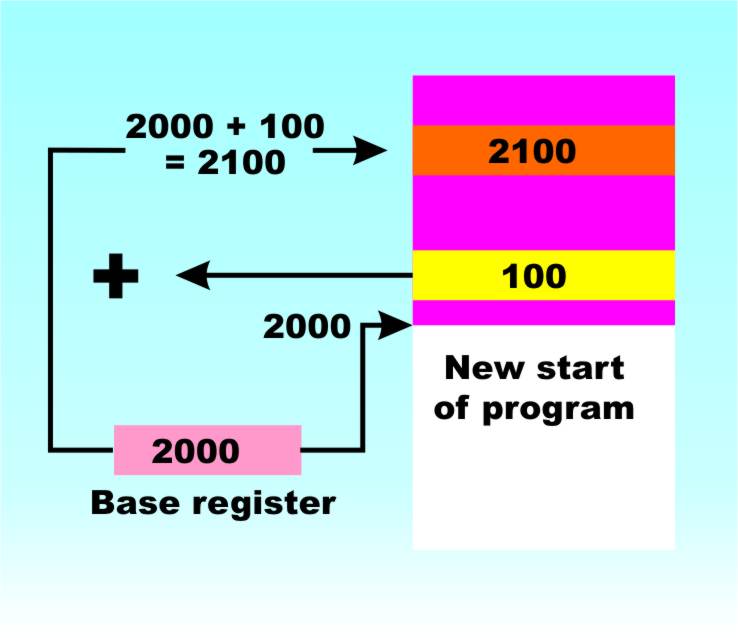
Partitions – optimisation for the computer Using partitions brings with it an interesting problem. The machine’s memory is usually addressed starting at 0000 and working up to the highest memory location. When a program is written the programmer usually assumes that it will be loaded starting at a particular location – 0000 say. Now think about what partitioning does to this assumption. If the first partition is full and a program is loaded into the second partition starting at 10000 say, then all its addresses are wrong and it isn’t going to work. The simplest and first solution to this problem was to make the program loader, which is part of the operating system, adjust all addresses to be correct for the current “load point”. This is usually called a “re-locating loader” and, while this possible it is very expensive in time and effort. A better solution is to introduce a special “base register” and calculate all addresses are calculated relative to it. So if a program refers to memory location 0003 this really means “the base register’s contents plus 0003”. Now all the operating system has to do is load the base register with the starting address of the program, i.e. according to which partition it is loaded into, and it all works nicely. Base registers eventually evolved into “segmented addressing” hardware in which multiple base registers are available for code and data and so on. All Intel processors since the 286 have supported segmented addressing and early versions of Windows used it to load programs into different locations without needing a relocating loader but Windows 95 and later have given them up in favour of a simpler approach. The main trouble with segmented addressing is that it confuses the programmer! To make things simpler the Win32 kernal, in use in all modern versions of Windows, uses flat addressing which means that every application has a complete address space and segments are forgotten - the segmentation hardware is still there but not used.
Base addressing makes re-location easy
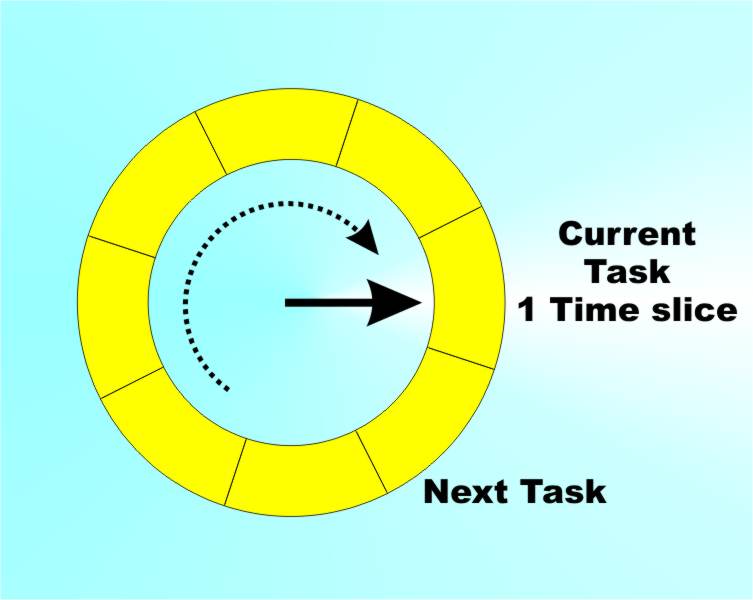
Of course, after a while playing with batch processing systems, we all wanted individual attention and our own VDUs connected directly to the machine and a copy of Star Trek or online chess or whatever. In this new world what was important was the user’s time not the computer’s time. Now we had to have multiple programs loaded and running so that they all appeared to be running at the same time. If at all possible each user had to be conned into thinking that they had the whole machine to themselves. This is the start of the more modern implementation of multitasking that leads up to desktop operating systems such as Windows 95/98 and later - although it has to be said that Windows isn’t a particularly good example of the art. So how does this magic actually work? Time slicingThe key to multitasking is time slicing coupled with good memory management. Time slicing simply makes use of the speed of a modern processor to make it look as if more than one thing is happening at a time. The operating system loads application programs one at a time into memory and maintains a list of active “tasks”. It then allocates a time slice – usually 1/10th of a second or thereabouts – to the first task in the list. When the time slice is up then the next application in the list gets a time slice allocated to it and so on until all of the applications in the list have had a time slice and the process starts over at the beginning of the list. Because of the “going back to the beginning” behaviour this processor management scheme is called a “Round Robin”. If any task is engaged in an I/O operation then it can be placed into a suspended state and miss its turn in the Round Robin until it is ready to do something again. In this way the time that a task would spend waiting for something to happen can be put to good use. You can also see that processes could be allocated priorities that control how many time slices they should be given each time around. This notion of priority can become very complicated but most systems distinguish three classes of priority – background (lowest), foreground (normal) and real time (highest).
Round Robin scheduling <ASIN:032143482X> <ASIN:0201442345> <ASIN:1847197108> |
|||
| Last Updated ( Friday, 10 June 2022 ) |