|
Page 1 of 3 A lightning guide to the basic ideas of computational complexity without the maths or the proofs. It's almost more fun than programming!
A Programmers Guide To Theory
First Draft
There is a more recent version of this:
Now available as a paperback and ebook from Amazon.

Contents
- What Is Computable?
- Finite State Machines
- What is a Turing Machine?
- Computational Complexity
- Non-computable numbers
- The Transfinite
- Axiom Of Choice
- Lambda Calculus
- Grammar and Torture
- Reverse Polish Notation - RPN
- Introduction to Boolean Logic
- Confronting The Unprovable - Gödel And All That
- The Programmer's Guide to Fractals
- The Programmer's Guide to Chaos*
- Prime Numbers And Primality Testing
- Cellular Automata - The How and Why
- Information Theory
- Coding Theory
- Kolmogorov Complexity
*To be revised
Computational complexity, roughly speaking how difficult a problem is to solve, has turned out to be an area of study that has revolutionised the way that we think about the world.
Forget relativity, black holes and the origins of time; computing has provided us with an incredible perspective on the universe of what we can and cannot know.
In case you are thinking that this stuff is insubstantial theorising, it isn't and every programmer should know something about complexity theory just to avoid having to spend the rest of time trying to work something out that `looks' easy.
This is a "beginner's" overview designed to get you started on the subject. You need to be warned that it gets a lot more subtle and confusing as you press on into other definitions of complexity - but to start at the very beginning.
Orders
The easy part of complexity is already known to most programmers as how long it takes to complete a task as the number of elements increases. You most often come across this idea in connection with evaluating sorting and searching methods but it applies equally well to all algorithms.
If you have a sorting method that takes 1 second to sort 10 items how long does it take to sort 11, 12 and so on items. More precisely what does the graph of sort time against n, the number of items look like?
You can also ask the same question for how much memory an algorithm takes and this is usually called its space complexity to contrast with the time complexity that we are looking at.
If you plot the graphs of time against n for a range of sorting methods then you notice something surprising. For small n some sorting methods will be better than others and you can alter which method is best by `tinkering' with it, but as n gets larger your tinkering gets swamped by the real characteristic of the method.
If you look at Figure 1 you will see what I mean. It is how fast the graph increases with n that matters because if one curve is rising more steeply than another it doesn't matter how they start out there will always be a value of n that makes the first curve bigger.
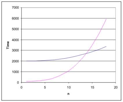
Figure 1: Orders of running time
This rate of increase in time with n is usually described by giving the rough rate of increase in terms of powers of n.
For example, a graph that increases like a straight line is said to be of order n - usually written O(n) and graph that increases like n squared is said to be order n squared or O(n2) and so on...
Obviously if you have a choice of methods then you might think that you should prefer the lowest order method you can find, but this is only true if you are interested in large values of n. For small values of n an elaborate method that proves faster for large values of n may not do as well.
In mathematical terms for small n the constants and lower order powers might matter but as n gets bigger the highest power term grows faster than the rest and eventually dominates the result.
So we ignore all but the highest power or fastest growing term and throw away all the constants to report the order of an algorithm.
In the real world often these additional terms are important and we have to put them back in. In particular when comparing algorithms at a fine level the lower terms and even constants are useful.
It is interesting to ask what makes one algorithm O(n), another O(n2) and so on?
The answer lies in the loops.
If you have a single loop that processes a list of n elements then it isn't difficult to see that it runs in time O(n). If you nest one loop inside another you get O(n2) and so on. In other words, the power gives you the maximum depth of nested loops in the program and this is the case no matter how well you try to hide the fact that the loops are nested! You could say that an O(nm) program is equivalent to m nested loops. This isn't a precise idea - you can always replace loops with the equivalent recursion for example but it sometimes helps to think of things in this way.
As well as simple powers of n, algorithms are often described as O(log n) and O(n log n) (where log is usually to the base 2). These two, and variations on them, crop up so often because of the way some algorithms work by repeatedly `halving' a task.
For example, if you want to search for a value in a sorted list you can repeatedly divide the list into two - a portion that certainly doesn't contain the value and a portion that does.
This is the well known binary search. If this is new to you then look it up because it is one of the few really fundamental algorithms.
Where does log n come into this?
Well ask yourself how many repeated divisions of the list are necessary to arrive at a single value. If n is 2 then the answer is obviously 1 division, if n is 4 then the answer is 2, if n is 8 then the answer is 3 and so on. In general if n=2m then it takes m divisions to reach a single element.
As the log to the base 2 of a number is just the power that you have to raise 2 to get that number, i.e. log2 n = log2 2m=m, you can see that log2 n is the just the number of times that you can divide n items before reaching a single item.
Hence log2 n and n log2 n tend to crop up in the order of clever algorithms that work by dividing the data down. Again you could say that an O(log2 n) algorithm is equivalent to a repeated halving down to one value and O(nlog2 n) is equivalent to repeating the partitioning n times to get the solution.
As this sort of division is typical of recursion you also find O(log2 n) a mark of a recursive algorithm.
When a recursive algorithm runs in O(nx) it is simply being used as a way of covering up the essentially iterative nature of the algorithm!
Why I waited years...
You may not think that the order of an algorithm matters too much but it makes an incredible difference.
For example, if you have three algorithms one O(n), one O(n log2 n) and one O(n2) the times for various n are:
| n |
O(n) |
O(n log2 n) |
O(n2) |
| 10 |
10 |
33 |
100 |
| 100 |
100 |
664 |
10000 |
| 500 |
500 |
4483 |
250000 |
| 1000 |
1000 |
9966 |
1000000 |
| 5000 |
5000 |
61438 |
25000000 |
If you want a more practical interpretation of these figures consider them as times in seconds. When you first develop an algorithm, testing on 10 items reveals a spread of times of 10 seconds to about 1.5 minutes using the different algorithms . If you move on to 5000 cases the difference is 1.4 hours for the O(n) to around three quarters of a year for the O(n2) algorithm!
In the case of an O(n!) algorithm a value of n equal to just 100 items gives a number with over 150 digits and a time that is longer than the age of the universe by quite a bit!
If you think that this sort of mistake never happens then I can tell you it does.
When I first started programming I implemented what I thought was a very reasonable graphics algorithm that worked by sorting co-ordinates. It wasn't that wasn't fast on the test data of tens of cases but it was acceptable.
When it came to running it on a real data set with hundreds of points all that happened was that the machine went dead - for hours.
At first I thought the program or machine had crashed and went into debug mode. Some time later when I had traced through hundreds of perfect loops the light dawned that it really was working OK but it would take something like ten years to finish!
Complexity matters.
<ASIN:0521424267>
<ASIN:0201000237>
|