| How To Draw Einstein's Face Parametrically |
| Written by Mike James | |||||
| Thursday, 19 July 2018 | |||||
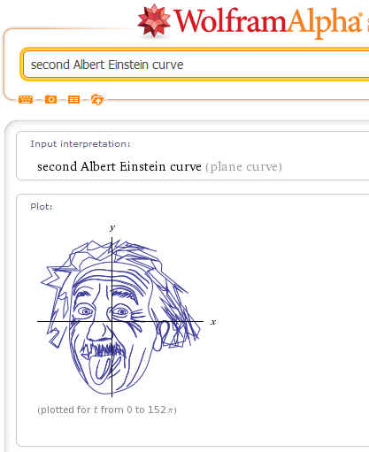
Page 1 of 4 There are some amazing math artworks on Wolfram Alpha. I was captivated by parametric equations that draw the faces of well known people and all using a few Sin functions. How is this achieved? It seems like a lot of work to go to if the curves are constructed by manual trial and error. The good news is that they are not - we show you how using Wolfram and Python. First we need to look at what people have produced. If you go to Wolfram Alpha and search for "person curve" you will discover that are more than 140 examples of these mathematical portraits. A popular and fairly typical one is of Albert Einstein:
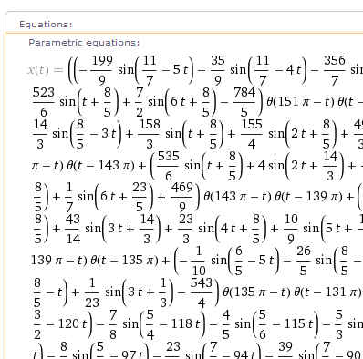
What you are looking at is an x, y plot of a pair of functions. If you look at the Equations window below the plot you will see that these are no simple functions:
Someone spent days or months handcrafting equations that produce the portraits in mathematical form - or did they? If you are going to produce a mathematical equation then presumably you know some math and math can always help you eliminate tedious work - unless, that is, you are still at the stage of confusing math with arithmetic. There is a mathematical procedure for producing these equations and it isn't that difficult, even though it does involve some reasonably advanced ideas. Let's find out how it all works by way of first a simple illustration using Mathematica and then an equivalent Python program. Parametric equationsFirst what is a parametric equation? Standard graphs simply plot one value of y for each value of x and clearly this is not what is happening here. To create graphs that have multiple values of y for each value of x you have to do things slightly differently and this is where parametric functions come in. A pair of parametric functions give you a value fo x and a value of y for each value of their parameter. That is
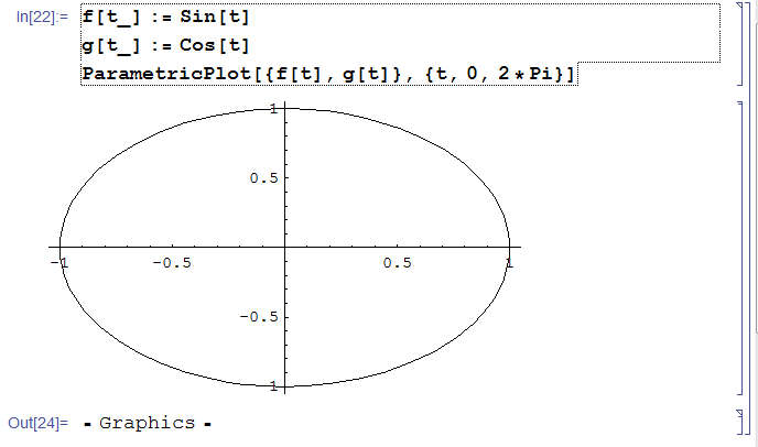
To create a plot all you have to do is take different values of t and plot the resulting x and y values. For example in Mathematica you can write:
And a plot will be drawn of all the x,y pairs for t from 0 to 2*Pi and the result is a circle (allowing for distortion due to the aspect ratio):
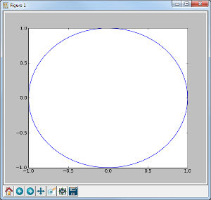
You can create the same plot in Python as long as you have MatPlotLib, Numpy and/or SciPy installed.
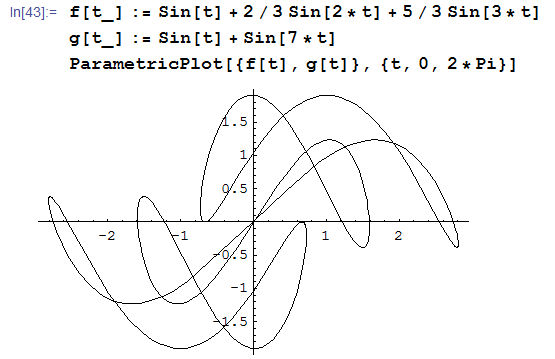
If you vary the mix of trigonometric functions you can create closed curves with complicated shapes. For example:
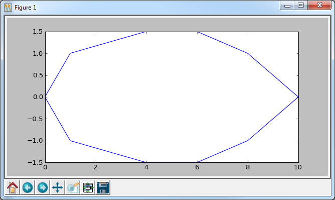
So our problem now is to work out a combination of Sin functions of different amplitudes and frequencies to change the complex but messy curve above into something that looks like Einstein. This is not going to be easy. First, digitize your curveNo doubt if you spend a lot of time on the problem you will eventually pick up some intuitions into how to create shapes of particular types. Eventually you could put together a toolkit of shapes that you could use to make other shapes - but this doesn't sound like a good way to spend your creative talent. The easy way to do the job is to start of with a digitization of the curve you want to create. You can obtain this by manually measuring a photo using Photoshop or Gimp or you could use a filter that automatically converts the grey scale photo to a line drawing. Alternatively if you really do have some artistic talent you could actually sketch the line drawing you want to turn into a parametric curve. As I don't have any talent, I'm going to use a crude digitization of an eye shape to show you how things work. I'm also not going to cover how to use or create a line filter.
|
|||||
| Last Updated ( Friday, 20 July 2018 ) |