| A Simple Discount Scheme |
| Written by Janet Swift |
| Friday, 30 October 2009 |
|
Spreadsheets such as Microsoft Excel and OpenOffice Calc can automate lookups making it possible to retrieve data easily. Here we use a look-up table to implement a simple discount scheme. 
Using lookup functionsLooking things up in tables is something we take for granted. We learn how to use lists and schedules early on in life and most of us even master bus and rail timetables! The basic spreadsheet functions, VLOOKUP and HLOOKUP, deal with data arranged in columns (i.e. vertically) and in rows (i.e. horizontally) respectively. There is also LOOKUP which handles only two-column (or two-row) tables but it is best avoided as it is limited in scope and functionality. Whichever orientation you choose for your table the first column or row contains the values (text or numbers) that you want to compare with a specified value and the second and subsequent ones contain the values that should be returned when a match is found. What happens when you use a lookup table is that the spreadsheet scans through a list, either of numbers or text, until it comes to an entry that is greater than the value that you have asked it to look up and then drops back one entry. This behaviour means that the list of values that are used to make this comparison, which are stored in the in the first column or row of the table, has to be in ascending order. Whether you are using the VLOOKUP or HLOOKUP function the syntax is basically the same. The function has three parameters (also referred to as arguments) enclosed between a set of parentheses and separated by commas. You can enter these by typing or pointing at cells or ranges in the spreadsheet. The first argument specifies the value to be looked up, the second the range used for the lookup table you have constructed and the third where to look. The third parameter is the offset value which specifies how many rows or columns to look below or to the left of the comparison values in the table. The row or column containing the comparison values is numbered as 1 and the values to be returned start in row or column 2.
LOOKUP TABLES AT A GLANCE
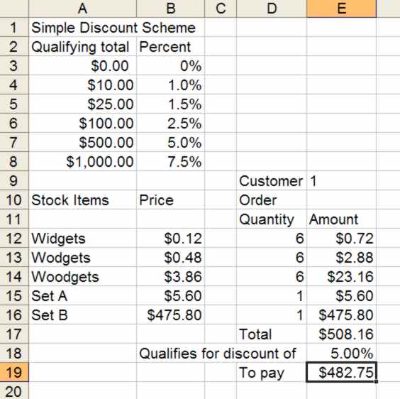
Spend more, save moreFor a simple example of the use lookup tables let's consider a scheme in which customers qualify for increasing discounts as they spend more. It could equally well be used for calculating sales commission or points earned in a rewards scheme. The spreadsheet we are aiming to construct is:
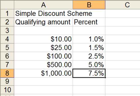
The idea is that the user can enter the customer number and the number of each stock item ordered. The spreadsheet then works out the total price, the discount and the final price after applying the discount. To take the effort out of following this step-by-step you can download a skeleton spreadsheet that contains all the labels and basic data. Or if you prefer to start from scratch type in the titles and labels, the qualifying amounts $10, $25, $100 and so on into column A, starting in cell A4 and the corresponding discounts into column B starting in cell B3 - as shown below:
We want to display percentages in column B and the easiest way to enter them is to type the percentage sign after each value - i.e. type in 1%, 1.5%, 2.5%, 5%, 7.5%. If you prefer to type in raw values and then format the cells to display percentages enter decimal fractions, i.e. 0.01 for 1%. Next we need to add a list of stock items and their prices and an area in which customer's orders can be entered as shown below.
The formula to calculate the amounts spent on the first item is =D12*B12 i.e. Price X Quantity. This needs to be copied down the column. We also need to compute the total cost, i.e. the sum of all the Amounts, and this is just a matter of entering the formula =SUM(E12:E16) in E17. Next we need some example data to see the spreadsheet in action. Enter the quantities of each item ordered by our first customer as shown here in the column labeled "Quantity":
For these example figures the order total computed by the SUM function in E16 is $508.16. If you inspect the discount table by eye you will see that this qualifies for a discount of 5% but we want the spreadsheet to return the discount.
The formula to enter in D18 to lookup the corresponding level of discount is: =VLOOKUP(E17,A4:B8,2) If you enter this and press the Enter key you will see 0.05 (i.e. 5%) appear. However the default currency formatting is confusing. To remedy this by displaying it as a percentage right-click cell D18, select Format Cells from the popup menu and select Percentage from the list.
Next we need a formula to apply the discount returned by the Lookup function to the total. Enter in E19: =E17*(1-D18) This reduces the total by the percentage by multiplying by 1 minus the discount percentage – i.e. by 0.95 or 95% in this case . Now it all seems to work but there is a small problem. Suppose the next customer only buys 40 widgets giving a total of $4.80. As this is less than $10 there isn’t a discount to apply and this leads to #N/A being displayed in both D18 and E19.
The way to avoid this type of error message and to compute the discount correctly is to ensure that the lookup table covers all the possibilities - including the ones at the ends of the range. In this case we missed out anything below $10. To include these lower amounts we need to extend the table down to zero. To do this type 0 in A3 and 0% (or just 0) in B3 and edit the formula in D18 to refer to the table range A3:B8 making it read =VLOOKUP(H8,A3:B8,2). This will result in 0% being displayed in D18 and the total of $4.80, i.e. no discount has been applied, being repeated in D19. The spreadsheet is now complete and works as expected.
<ASIN:0750681853> <ASIN:0470046554> <ASIN:0470044039>
|
| Last Updated ( Friday, 16 April 2010 ) |