| The Ultimate Guide to Pivot Tables for Beginners |
| Written by Hannah Sharon | ||||
| Monday, 15 July 2019 | ||||
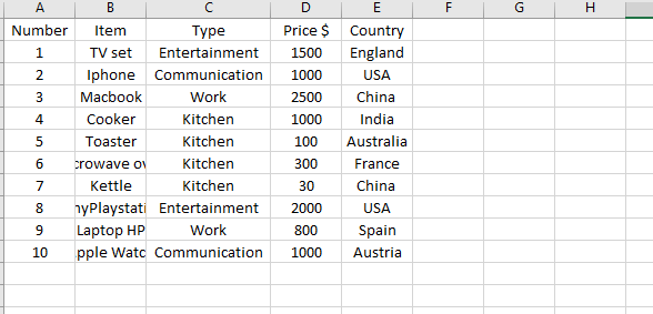
Page 1 of 3 Pivot tables are one of Excel's most powerful features. Used in the context of data processing a Pivot table can be used to summarize, sort, reorganize, group, count, total or average data stored in a database. For time-saving, efficient pivot tables that help create outstanding reports, here’s the ultimate guide to using pivot tables. Before you start reminiscing about that episode on Friends where Ross yells “Pivot!” while trying to manoeuvre a couch through the hallway, I need to reveal that a pivot table is, in fact, a tool in Excel, and not an actual table you have to pivot. It enables you to summarize selected columns and rows of data in a spreadsheet in order to arrive at a pristine and highly organized report the Excel gods at Spreadsheeto would be proud of. Easy formulas and neat reports in half the timeA pivot table is a great formula allows grouping data — choose a field, any field! It’s sure to set things in order with a few clicks here and there. Pivot tables are the perfect solution for when you’re in need of ironing out large groups of data. A good report is anything but messy. A good report is laid out neatly, easy on the eyes, and is presentable and clear. With a well-made pivot table, you do exactly that. Using pivot tables is a very important Excel skill to learn. First, you need a spreadsheet with data like this one with sold appliances/their price/country where they are shipped to/their categories:
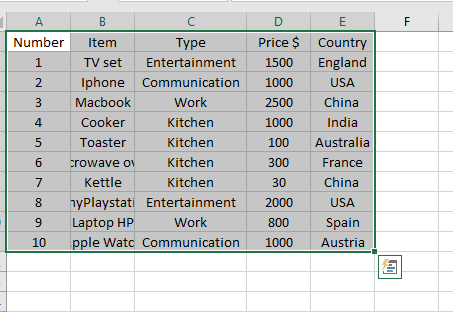
Step 1: Select the items you wish to analyse or group together Click on the corners of the cells you’d like to work on and drag your mouse over the selected area. Selecting the cells — including their respective column headers — will highlight the data you’d like to work with:
Step 2: Select the “Pivot Table” command Coming from the toolbar, select the Insert tab. This section will reveal the Pivot Table command:
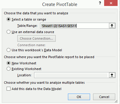
Step 3: Explore the Pivot Table The Create Pivot Table dialogue box will appear. From here, you may choose your settings, then click on OK:
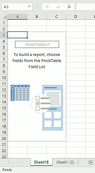
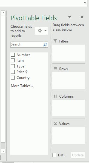
A blank Pivot Table and Fields will appear on a new worksheet for you to explore:
|
||||
| Last Updated ( Monday, 15 July 2019 ) |
